


Short Summary
A property market forecast is only as good as the data and methodology behind it. HtAG Analytics has built a 3-method composite statistical model — drawing on momentum-decay, weighted CAGR blending, and mean-reversion analysis — to project 12-month typical price growth across all eight Australian states and territories. Powered by 2,327,175 monthly observations spanning January 2010 to February 2026, this forecast reveals a market in broad deceleration, with composite growth projections ranging from 4.3% in Victoria to 10.6% in Western Australia.
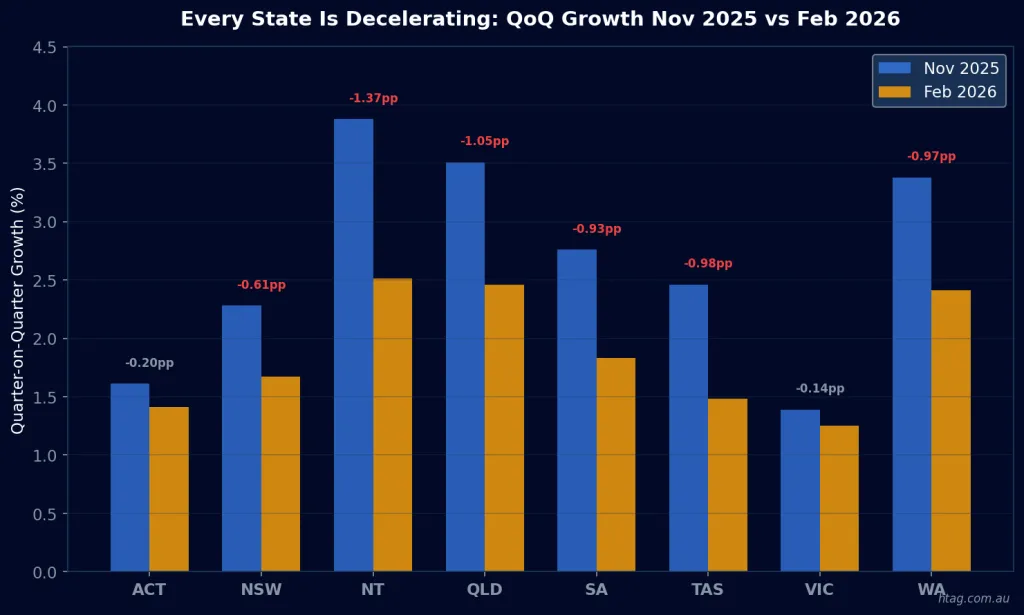
The National Picture: Broad Deceleration, Uneven Landing
The Australian residential property market in early 2026 is characterised by a broad deceleration phase following the post-pandemic boom. According to HtAG Analytics data, the national typical 3-bedroom house price sits at approximately $835,000 as of February 2026, with trailing 12-month annualised growth rates varying from 4.5% in Victoria to 14.1% in Western Australia. However, this headline figure masks enormous variation between states — and critically, the quarterly growth rate is falling in nearly every jurisdiction.
The deceleration is unmistakable. Between November 2025 and February 2026, quarter-on-quarter growth rates fell in seven of eight states. Queensland’s annualised 3-month momentum dropped from 12.9% (trailing 12-month) to 9.3% (trailing 3-month). Western Australia fell from 14.1% to 9.9%. South Australia slowed from 9.3% to 7.3%. Even the annual growth numbers, which still look robust in headline terms, are increasingly built on momentum from earlier in the cycle rather than current-quarter strength.
According to HtAG Analytics’ analysis of 2,327,175 monthly observations across 4,881 Australian suburbs, nearly every state is decelerating from its post-pandemic peak growth rate — but the magnitude and timing of this deceleration varies dramatically, creating distinct investment windows across the country.
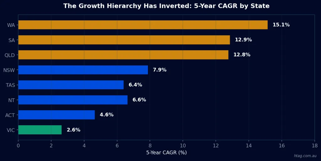
What makes this cycle particularly significant is the inversion of Australia’s traditional growth hierarchy. Western Australia, Queensland, and South Australia — historically considered secondary markets — have delivered 5-year compound annual growth rates (CAGRs) of 15.1%, 12.8%, and 12.9% respectively. Meanwhile, Victoria has recorded just 2.6% over the same period, well below its long-run 10-year average of 5.2%.
This growth hierarchy inversion is not permanent — it never is. Historical analysis shows that Australian property markets are cyclical and asynchronous. The states that lead one cycle often lag the next. Understanding where each state sits in its cycle is essential for timing investment entry.
How Were These Property Forecasts Generated?
HtAG Analytics’ 12-month property forecasts are generated using a 3-method composite statistical model. Rather than relying on a single forecasting approach — each of which carries inherent biases — we blend three independent methodologies and average their outputs to produce a more robust central estimate. The three methods are:
Method 1: Momentum with Decaying Deceleration
This method takes the current trailing 12-month annualised growth rate and adjusts it for observed deceleration (or acceleration) over the past two quarters. The deceleration signal is applied with an exponential decay, acknowledging that recent momentum shifts may partially reverse. This method is most responsive to current market conditions.
Method 2: Weighted CAGR Blend
This method blends growth rates across three time horizons — 50% weight on the trailing 12-month annualised rate, 30% on the 5-year CAGR, and 20% on the 10-year CAGR. By incorporating long-run structural growth rates alongside recent performance, this approach anchors the forecast to fundamental trends while still capturing current dynamics.
Method 3: Mean-Reversion Model
This method assumes that above-trend or below-trend growth rates will partially revert toward the long-run average. It applies a 70% weight to current momentum and 30% to the 10-year long-run growth rate. This method provides the most conservative estimates for boom-phase markets and the most optimistic for lagging markets like Victoria.
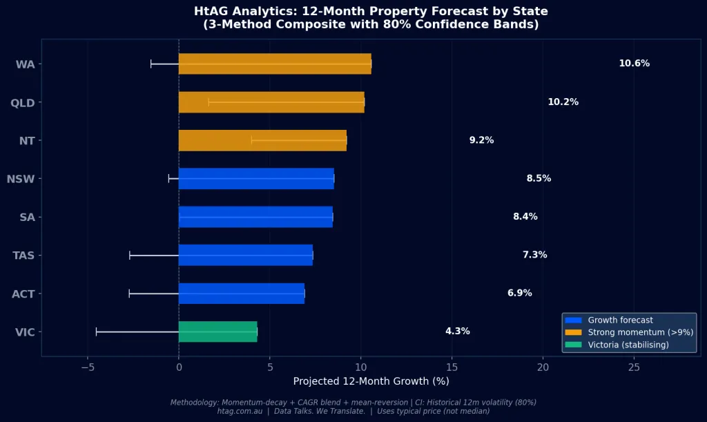
HtAG Analytics’ 3-method composite forecast blends momentum-decay, weighted CAGR, and mean-reversion models across 2.3 million data points. The 80% confidence intervals are derived from each state’s historical 12-month return volatility, providing a statistically grounded range of outcomes.
The composite forecast is the equal-weighted average of all three methods. Confidence bands are calculated using each state’s observed historical volatility in 12-month returns, producing an 80% probability interval — meaning there is roughly an 80% chance the actual outcome falls within the stated range, assuming historical volatility patterns persist.
State-by-State 12-Month Property Forecasts (March 2026 – February 2027)
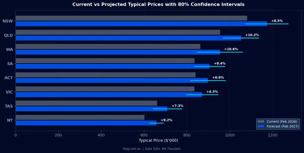
The table below presents HtAG Analytics’ composite 12-month growth forecast for the typical 3-bedroom house price in each Australian state and territory. The “Low” and “High” columns represent the 80% confidence interval bounds.
| State | Current Typical Price | Composite Forecast | Low (80% CI) | High (80% CI) | Projected Price |
|---|---|---|---|---|---|
| WA | $862,792 | 10.6% | -1.5% | 22.6% | $953,837 |
| QLD | $954,746 | 10.2% | 1.6% | 18.8% | $1,052,018 |
| NT | $602,184 | 9.2% | 4.0% | 14.4% | $657,630 |
| NSW | $1,081,037 | 8.5% | -0.6% | 17.6% | $1,173,008 |
| SA | $835,290 | 8.4% | 0.0% | 16.8% | $905,800 |
| TAS | $660,560 | 7.3% | -2.7% | 17.4% | $709,027 |
| ACT | $839,887 | 6.9% | -2.7% | 16.5% | $897,866 |
| VIC | $834,600 | 4.3% | -4.5% | 13.1% | $870,413 |
Source: HtAG Analytics. 3-method composite model applied to AUS-TS dataset. Typical prices as of February 2026. 80% confidence intervals based on historical 12-month return volatility.
The Standouts: WA and QLD
Western Australia leads the composite forecast at 10.6%, closely followed by Queensland at 10.2%. Both states carry strong momentum from the past two years, but the wide confidence intervals (WA: -1.5% to 22.6%; QLD: 1.6% to 18.8%) reflect elevated volatility and the genuine possibility that deceleration could be sharper than the base case suggests. WA’s 5-year CAGR of 15.1% is the highest in the country, but its trailing 3-month annualised rate has already dropped to 9.9% — a clear deceleration signal.
The Northern Territory Surprise
The NT records the third-highest composite forecast at 9.2%, with the tightest confidence interval of any state (4.0% to 14.4%). This reflects a combination of strong recent momentum and low historical volatility. However, the NT’s small sample size (fewer tracked suburbs) means this estimate should be interpreted with additional caution.
The Contrarian: Victoria
Victoria is the most interesting market in this dataset. Its composite forecast of 4.3% is the lowest nationally, yet the direction of momentum is turning positive. Victoria’s trailing 3-month annualised rate (4.3%) has risen above its trailing 12-month rate (4.5%), and the deceleration metric has turned modestly negative (-1.2pp), suggesting the bottom of the cycle may be forming.
HtAG Analytics data shows Victoria’s 5-year CAGR of just 2.6% sits well below its 10-year average of 5.2%, suggesting significant mean-reversion potential. Victoria is the standout contrarian opportunity in the 2026 property forecast landscape.
Victoria’s price-to-rent ratio of 30.7x and expanding yields (+31 basis points since 2021) create a fundamentally different risk-return profile compared to the yield-compressed boom states. For investors with a 5–10 year horizon, Victoria’s position today resembles where Western Australia and Queensland were in 2019–2020 — before their boom cycles began.
What Is Yield Compression and Why Does It Matter in 2026?
Yield compression occurs when property prices rise faster than rents, reducing the gross rental yield available to new buyers. It is one of the most critical — and most overlooked — dynamics in the current Australian property market. Every state except Victoria has experienced significant yield compression since 2021.
| State | Yield 2021 | Yield Feb 2026 | Change (bps) | Price-to-Rent Ratio |
|---|---|---|---|---|
| QLD | 4.24% | 3.14% | -110 bps | 31.8x |
| WA | 4.50% | 3.54% | -96 bps | 28.2x |
| SA | 4.29% | 3.38% | -92 bps | 29.6x |
| NT | 5.81% | 5.18% | -63 bps | 19.3x |
| ACT | 4.09% | 3.77% | -33 bps | 26.5x |
| NSW | 3.23% | 2.90% | -33 bps | 34.5x |
| TAS | 4.28% | 3.96% | -32 bps | 25.3x |
| VIC | 2.94% | 3.25% | +31 bps | 30.7x |
Source: HtAG Analytics. Yield = annual rent ÷ typical price. Data as of February 2026.
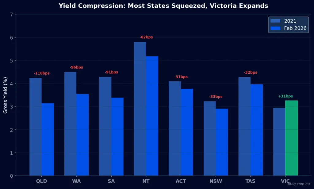
According to HtAG Analytics data, Queensland has experienced the sharpest yield compression in Australia since 2021 — a fall of 110 basis points — meaning new investors are paying significantly more per dollar of rental income than those who entered five years ago.
Victoria stands alone as the only mainland state where yields have expanded (+31 basis points). Typical prices softened while rents grew — a classic contrarian income-investor entry signal. For yield-focused investors, Victoria’s current 3.25% gross yield may not sound exciting in isolation, but the direction of travel (expanding) is the opposite of every other state (compressing).
A critical statistical finding from HtAG’s analysis: the correlation between price growth and rent growth at suburb level is near-zero (Pearson r = 0.007). Capital growth and rental yield are largely independent objectives — pursuing both from a single property is statistically unlikely. This means investors must choose their primary objective and select suburbs accordingly.
Where Does Each State Sit in the Property Market Cycle?
Market cycle analysis classifies each state based on the direction and rate of change in quarterly price growth. Australian property markets are cyclical and asynchronous — no state is permanently hot or cold. They rotate through growth cycles with different timing and amplitude, creating opportunities for investors who understand the cycle rather than chasing recent performance.
Based on HtAG Analytics’ momentum and deceleration analysis, the current cycle phases are:
- Late Boom / Early Deceleration (WA, QLD, SA) — Still growing above long-run averages but momentum is clearly fading. These states carry the highest growth forecasts but also the widest confidence intervals and greatest risk of sharper-than-expected slowdowns.
- Mid-Deceleration (NSW, NT, TAS) — Growth rates are moderating toward long-run averages. These markets are transitioning from boom to normalisation and offer a more balanced risk profile.
- Stabilisation / Early Recovery (ACT) — Growth has modestly accelerated, with the deceleration metric near zero. ACT appears to be finding a stable growth floor.
- Trough / Contrarian Entry (VIC) — The only state where momentum has turned positive. Victoria’s position today resembles where WA and QLD were in 2019–2020, before their boom cycles began.
The historical pattern is instructive. The Sydney/Melbourne boom of 2013–2017 saw NSW and VIC experience sustained double-digit growth while WA was declining. The pandemic boom of 2021–2022 saw every state participate. The current phase (2024–2026) has rotated growth to WA, QLD, and SA. For cycle-timing investors, understanding these rotations is more valuable than any single-year forecast.
245 No-Go Suburbs: Where the Data Says to Avoid
Not all growth is good growth, and not all suburbs warrant investment. Across the 1,379 high-confidence suburbs in HtAG’s dataset (filtered for 20+ sales and 10+ rentals in the trailing 12 months), 245 suburbs — 18% of the total — have been flagged as no-go zones across four distinct risk categories:
- Peaked Markets (57 suburbs) — High trailing growth but momentum decelerating sharply, with yields compressed below 4%. These are the suburbs most at risk of price correction as the growth cycle fades.
- Yield-Trapped (180 suburbs) — Gross yield below 2.5%, concentrated in inner Sydney (99 suburbs), Melbourne (36), Brisbane (30), and Perth (15). These suburbs require exceptional capital growth just to match risk-free returns.
- Declining & Decelerating (5 suburbs) — Active price correction with no sign of bottoming. Negative growth with negative momentum — the worst combination.
- Overheated (13 suburbs) — Growth above 25% per annum, two to three standard deviations above the national average. Statistically unsustainable and at elevated correction risk.
HtAG Analytics has identified 245 no-go suburbs (18% of high-confidence suburbs) across four risk categories. The full suburb-level list is available in HtAG’s complete Australian Residential Property Statistical Analysis White Paper, exclusively available to Professional subscribers.
The full suburb-level no-go zone list, along with specific investment opportunity shortlists across three risk-return categories (high-growth momentum, balanced growth-yield, and contrarian deep-value), is available in HtAG Analytics’ complete Australian Residential Property Statistical Analysis White Paper, exclusively available to Professional subscribers.
How HtAG Analytics Powers This Forecast
This forecast is powered by HtAG Analytics’ proprietary AUS-TS dataset — 2,327,175 monthly observations spanning January 2010 to February 2026, covering 4,881 suburbs across all eight states and territories. The dataset tracks typical prices (not simple medians — learn why typical price is more reliable), rental yields, sales volumes, rental volumes, and growth rates at multiple time horizons.
The forecasting methodology employs the 3-method composite approach described above, along with CAGR calculations, momentum detection, Pearson and Spearman correlation analysis, historical volatility estimation, and market cycle classification. Every number in this article is derived from statistical analysis — not opinion, not sentiment, and not cherry-picked anecdotes.
HtAG’s platform gives investors and buyers agents access to GeoDex for suburb-level heatmap analysis, the Growth Rate Cycle (GRC) for market timing, Market in Motion (MiM) for interactive data exploration, and the Evidence Portal which tracks 135+ validated property recommendations with documented performance outcomes.
Key Takeaways
- HtAG Analytics’ 3-method composite model forecasts 12-month typical price growth ranging from 4.3% (VIC) to 10.6% (WA), with wide 80% confidence intervals reflecting genuine uncertainty in a decelerating market.
- Nearly every state is decelerating. WA’s trailing 3-month annualised rate has dropped to 9.9% from a 12-month rate of 14.1%, and QLD’s has fallen to 9.3% from 12.9% — clear momentum fade signals.
- The traditional growth hierarchy has inverted: WA (15.1%), SA (12.9%), and QLD (12.8%) 5-year CAGRs are 2–6x higher than Victoria’s 2.6%, but this divergence is historically temporary.
- Victoria is the standout contrarian opportunity — the only state with positive momentum, expanding yields (+31 bps since 2021), and a 5-year CAGR well below its long-run average.
- Rent growth has stalled nationally, and the near-zero correlation (r = 0.007) between price and rent growth means capital growth and yield are independent objectives — choose one.
- 245 no-go suburbs identified (18% of high-confidence suburbs) across peaked, yield-trapped, declining, and overheated categories. Full suburb lists available to HtAG subscribers.
FAQs
HtAG Analytics’ 3-method composite model forecasts 12-month typical price growth ranging from 4.3% in Victoria to 10.6% in Western Australia as of March 2026. The national picture is one of broad deceleration — most states are still growing but at declining rates. Western Australia and Queensland lead on absolute growth, while Victoria offers the strongest contrarian entry signal with positive momentum off a low base.
Western Australia has the highest composite growth forecast at 10.6%, followed by Queensland at 10.2% and the Northern Territory at 9.2%. However, these states also carry the widest confidence intervals — WA’s 80% confidence band spans from -1.5% to 22.6% — reflecting elevated volatility and the possibility of sharper-than-expected deceleration. According to HtAG Analytics data, WA’s 5-year CAGR of 15.1% is the highest nationally.
Victoria is the standout contrarian opportunity in 2026. While its composite forecast of 4.3% is the lowest nationally, it is the only state where momentum has turned positive and yields are expanding (+31 basis points since 2021). HtAG Analytics data shows Victoria’s 5-year CAGR of 2.6% is well below its 10-year average of 5.2%, suggesting significant mean-reversion potential for patient investors with a 5–10 year horizon.
A typical price is HtAG Analytics’ preferred metric for measuring property values at suburb level. Unlike a simple median (the middle value of all sales), the typical price methodology accounts for composition bias — for example, when a suburb’s sales mix shifts between houses and units, or between different bedroom counts. HtAG explains in detail why typical price is more reliable than median price for investment analysis.
HtAG Analytics’ AUS-TS dataset covers 4,881 suburbs with 2,327,175 monthly observations from January 2010 to February 2026. For the state-level forecasts in this article, suburb-level typical prices were aggregated to state medians. The no-go zone analysis used a high-confidence filter of 20+ sales and 10+ rentals in the trailing 12 months, reducing the sample to 1,379 suburbs with statistically reliable data.
See the Data Behind the Forecasts
Every forecast in this article was powered by HtAG Analytics — the same platform used by professional buyers agents across Australia. Explore GeoDex heatmaps, track suburb performance with the Growth Rate Cycle, and access the full Statistical Analysis White Paper with suburb-level forecasts, no-go zone lists, and investment shortlists.
Disclaimer: This article is for educational purposes only and does not constitute financial advice. Property investment carries risks, and past performance is not indicative of future results. All growth rates, yields, and projections are derived from historical data and statistical modelling — they are not guarantees of future performance. Always conduct your own due diligence and consult a qualified financial adviser before making investment decisions.


