


Table of Contents
- Quick Summary
- Why a Framework Beats a “Best Suburbs” List
- Step 1: Establish the Brief Before You Look at Data
- Step 2: Validate Demand Depth and Affordability
- Step 3: Read the Supply Picture
- Step 4: Read the Demand Picture
- Step 5: Score Growth Momentum
- Step 6: Stress-Test the Risks
- Step 7: Time the Entry
- Putting the Framework Together
- Key Takeaways
- From Data Signal to Portfolio Decision
- Frequently Asked Questions
Quick Summary
Analysing a suburb for investment means stress-testing it across seven measurable layers — supply, demand, growth momentum, affordability, socioeconomic depth, risk, and timing — rather than relying on median price snapshots or anecdotal “hot spot” lists. HtAG Analytics tracks more than 150 metrics across 15,000+ Australian suburbs to surface the small minority of markets that pass every layer. This guide walks through the framework data-driven investors and buyers agents apply before they shortlist a single property.
Why a Framework Beats a “Best Suburbs” List
Most property investors still analyse suburbs the same way they did in 2010: median price, recent growth, and a gut feel for the area. That approach now misses the structural drivers that separate a 12% capital-growth year from a 2% one. According to HtAG Analytics’ analysis of 15,000+ Australian suburbs, the median 5-year growth gap between top-decile and bottom-decile markets exceeds 60 percentage points — a gap that median price alone cannot explain.
A repeatable framework matters for three reasons. First, it removes confirmation bias — the tendency to fall in love with a suburb and then justify it with cherry-picked data. Second, it forces you to compare like with like across thousands of markets simultaneously, which the human eye cannot do. Third, it produces a written audit trail you can return to in twelve months to learn from your decisions.
The framework below is the same one used by HtAG Mastermind members and is grounded in HtAG’s Director’s Guidelines. Each step answers a specific question. Skipping any step means you’re investing without an answer to that question.
Step 1: Establish the Brief Before You Look at Data
Suburb analysis without a brief is the most common mistake new investors make. A brief defines the type of suburb you are looking for — long-term capital growth, mid-term balanced, short-term high-yield, or cashflow-first — before any data is opened.
The brief sets four parameters: timeframe (short, medium, long), risk tolerance (low, medium, high), budget band, and exit strategy (hold, recycle equity, sell). A suburb that scores brilliantly for a long-term low-risk buyer can score poorly for a short-term high-yield brief, and vice versa. A suburb is never “good” or “bad” in isolation — it is only ever a fit or misfit for a defined brief.
If you skip this step, you will end up overweighting whatever metric happens to look impressive on the day you ran your search. Investors who define the brief first finish their analysis with conviction; investors who don’t, finish with second-guessing.
Step 2: Validate Demand Depth and Affordability
Demand depth measures whether the buyer pool sitting behind a suburb’s current price is genuine or hollow. Two suburbs can have identical median prices and identical 12-month growth, yet one has years of incremental upside and the other is at its ceiling — the difference shows up in the affordability and income-quality data.
Three sub-checks belong in this step:
- Years to Own (YTO) — the multiple of household income required to purchase the median home. A YTO above 12 in regional markets, or above 15 in capital cities, signals affordability fatigue and limits future buyer migration.
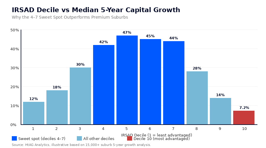
- IRSAD decile — the ABS Index of Relative Socio-economic Advantage and Disadvantage. HtAG Analytics’ research shows the IRSAD sweet spot for capital growth sits at deciles 4–7, where median 5-year growth historically reaches 44.5%, compared with 7.2% for decile-10 (most advantaged) suburbs. Premium suburbs already have their growth priced in.
- Owner-occupier ratio — a suburb dominated by renters is structurally more volatile. Owner-occupiers bid emotionally, hold longer, and absorb interest-rate shocks better than investors.
Cross-check all three. A suburb that looks affordable on YTO but sits at IRSAD decile 9 is a different proposition to one at decile 5 — the latter has a deeper buyer pool ready to bid prices forward over the cycle.
For a fuller treatment of why the median price you’re staring at can mislead you, see HtAG’s explainer on why median price is not a reliable metric for property investors.
Step 3: Read the Supply Picture
Supply is the most predictive single layer in suburb analysis because it is the slowest to change. Zoning, planning approvals, and developer pipelines move on multi-year timelines — which means a tight-supply suburb today is almost always a tight-supply suburb in eighteen months.
Four supply signals matter:
- Stock on Market (SOM) — total active listings. Falling SOM with stable demand is the cleanest bull signal in property data.
- Months of Supply — how long it would take to clear current listings at the current sales pace. Below three months is structurally tight; above six months is structurally loose.
- New dwelling approvals (LGA-level) — the pipeline of supply about to hit the market. A suburb inside an LGA with surging approvals will face headwinds even if its current SOM looks tight.
- Renter-Occupier ratio movement — a rising RO ratio in a previously owner-dominated suburb often precedes investor-led oversupply, especially in apartment-heavy precincts.
HtAG’s data shows suburbs in the bottom quintile for Months of Supply (tightest stock) outperformed the all-suburbs median by roughly 5 percentage points of capital growth over the following 12 months across the past decade. Supply scarcity is rarely priced in immediately — it leaks into prices over six to eighteen months.
Step 4: Read the Demand Picture
Demand depth from Step 2 told you whether the buyers exist. The demand picture in Step 4 tells you whether they are currently active. The two are related but distinct — many suburbs have deep latent demand that lies dormant until a trigger (interstate migration, infrastructure announcement, rate-cycle shift) wakes it up.
Three signals capture active demand:
- Days on Market (DOM) — falling DOM means buyers are competing harder. DOM below 30 days is intense; above 60 is weak.
- Auction clearance rate — sustained clearance above 70% in capital city suburbs signals active buyer competition.
- Search index momentum — buyer enquiry data from listing portals leads sales by four to eight weeks.
The cleanest signal is Days on Market falling at the same time Stock on Market is falling — that combination, which HtAG’s Bull-Bear Tide methodology calls a Bull Signal, has historically predicted +0.25 percentage points of forward 12-month growth above the suburb’s own trend. The opposite combination — DOM falling while SOM rises — is a Bear Signal, with -0.32 percentage points of forward underperformance.
For a deeper read of the property clock framework, see HtAG’s Growth Rate Cycle explainer.
Step 5: Score Growth Momentum
Growth momentum tells you which phase of the cycle a suburb is sitting in — early recovery, expansion, late expansion, or contraction. Buying in the wrong phase is the most expensive timing mistake an investor can make.
HtAG Analytics uses three momentum metrics in combination:
- GRC (Growth Rate Cycle) — direction and acceleration of year-on-year price change. Suburbs transitioning from plateau to acceleration historically outperform decelerating suburbs by 6–9 percentage points over the following 12 months.
- GPD (Growth Pattern Deviation) — gap between current growth and the suburb’s own historical average across 3, 5, and 10-year windows. Negative GPD is favourable: it means the market is underperforming its own history and has room to catch up.
- GSP (Growth Spillover Effect) — gap between suburb growth and LGA average growth. Negative GSP is also favourable: it indicates the suburb is lagging its LGA peers and has spillover catch-up potential.
The compound signal — GRC accelerating, GPD negative, GSP negative — is rare and powerful. Suburbs in this configuration that also pass Steps 2–4 are the ones that historically appear in HtAG’s top-performing recommendation cohorts.
Think of it as a suburb running below its own trend, below its neighbours’ trend, and turning the corner — three independent reasons to expect catch-up upside.
| Momentum Configuration | Interpretation | Forward Bias |
|---|---|---|
| GRC accelerating, GPD negative, GSP negative | Early-cycle, multiple catch-up signals | Strong upside |
| GRC accelerating, GPD positive, GSP negative | Mid-cycle, hot vs own history but lagging LGA | Moderate upside |
| GRC plateau, GPD positive, GSP positive | Cycle peak risk | Caution |
| GRC decelerating, GPD positive, GSP positive | Cycle peak passed | Avoid for capital growth |
Step 6: Stress-Test the Risks
Suburb analysis without a risk layer is incomplete. Risk is what separates a suburb that performed well over the last cycle from one that will perform well over the next.
The risk audit covers four dimensions:
- Market concentration — single-employer towns, mining-dependent regions, and tourist-only economies all carry concentrated cashflow risk. Diversified service economies are more resilient.
- Public housing concentration — suburbs with elevated public housing density historically show higher capital-growth volatility and slower price recovery after corrections.
- Insurance and climate risk — flood, bushfire, and cyclone overlays at the property and suburb level are now material to insurability and resale value. Insurance premiums in some risk-rated suburbs have doubled in five years.
- Legislative and tax risk — tenancy law shifts, land-tax thresholds, and short-stay regulation changes can alter cashflow assumptions overnight.
A no-go decision at this step saves you from buying a suburb that screens beautifully on growth metrics but carries tail risk that wipes out the gain in a single legislative or insurance shock.
Step 7: Time the Entry
Even the right suburb purchased at the wrong moment under-delivers. The timing layer answers a single question: is the directional regime right now favourable for entry?
Three windows determine timing:
- National cycle phase — accumulation, expansion, late expansion, distribution, or contraction. National regime sets the gravitational pull all suburbs fight against.
- State cycle phase — each state runs its own cycle, often six to twelve months out of phase with the national signal.
- Suburb-level Bull-Bear Tide — the within-suburb DOM/SOM divergence covered in Step 4.
Aligning all three is the holy grail. Most of the time you will not get all three lined up — at which point the discipline is to lower your conviction and reduce your exposure, not to override the data because the property looks attractive.
For a current read on national and state cycles, see HtAG’s Australian Property Forecast 2026.
Putting the Framework Together

The seven steps do not have equal weight in every analysis. The brief from Step 1 reweights everything that follows. A long-term low-risk brief gives Steps 2 and 6 disproportionate weight. A short-term high-risk brief leans hardest on Steps 4, 5, and 7. A cashflow brief reweights toward yield, vacancy, and rent momentum that sit underneath Steps 3 and 4.
What never changes is the order. Brief comes first. Demand depth and supply come before momentum, because momentum without underlying depth is froth. Risk comes before timing, because no entry window justifies an avoidable structural risk.
Investors who apply this framework end up rejecting roughly nine out of every ten suburbs they shortlist. That rejection rate is a feature, not a bug. The suburbs that survive seven layers of scrutiny are the small handful where the data lines up — and those are the suburbs HtAG Analytics’ Evidence Portal tracks with named, validated capital-growth outcomes.
To see how the framework plays out in real recommendations and outcomes, browse the HtAG Evidence Portal where 135+ validated suburb recommendations are tracked with measured 12-month results.
Key Takeaways
- A repeatable seven-step framework — brief, demand depth, supply, demand activity, momentum, risk, timing — eliminates confirmation bias and produces an auditable analysis trail.
- Demand depth and IRSAD-decile analysis matter more than median price; the IRSAD 4–7 sweet spot has historically delivered 44.5% median 5-year growth versus 7.2% for decile 10.
- Supply is the slowest-moving layer and the most predictive — Months of Supply below three is structurally tight and historically precedes outperformance.
- The compound momentum signal (GRC accelerating, GPD negative, GSP negative) is the strongest single configuration for forward 12-month outperformance.
- Risk and timing are non-negotiable final layers — a suburb that screens well but fails Step 6 or Step 7 is not investable, regardless of how attractive the property is.
- Buyers who apply all seven steps reject around 90% of suburbs they shortlist. That filtering ratio is the strategic edge.
From Data Signal to Portfolio Decision
You now have the framework. The bottleneck most investors hit is the data. Running seven layers manually across thousands of suburbs is a full-time research job, which is why most people give up at Step 2 and revert to median price comparisons. HtAG Analytics built GeoDex, Market in Motion, and the Suburb Growth Forecasts 2026 toolset specifically to compress this into a workflow you can run inside an hour.
If you want the same data layer the framework above is built on — covering 15,000+ Australian suburbs, updated quarterly, with GRC, GPD, GSP, IRSAD, supply-demand, and risk metrics already wired together — start with the HtAG Starter Plan. It is the most efficient way to move from “I have a framework” to “I have a shortlist.”
For investors working with a buyers agent, HtAG’s advisory services extend the framework into a direct-to-investor research engagement.
Frequently Asked Questions
How long does a proper suburb analysis take?
Using a structured data platform such as HtAG, a full seven-layer analysis takes thirty to ninety minutes per suburb. Without a platform — pulling data manually from ABS, listing portals, and council planning records — the same analysis takes eight to twelve hours and rarely covers all seven layers consistently. The data overhead is the main reason most investors short-circuit the framework, not lack of methodology.
What’s the difference between LGA-level and suburb-level analysis?
LGA-level data captures pipeline supply and broad migration patterns; suburb-level data captures the actual price and demand signal an investor will trade against. You need both. LGA data without suburb data misses the dispersion inside the LGA — two suburbs in the same LGA can show 8% growth gaps in the same year. For a deeper treatment, see HtAG’s LGA vs Suburb Analysis.
Can I rely on growth alone if a suburb is showing strong recent gains?
No. Recent strong growth is the most overvalued signal in property data because it is the easiest to see and the slowest to mean-revert. HtAG’s GPD metric exists precisely because suburbs running well above their own historical trend tend to give back gains over the following one to three cycles. Strong recent growth without negative GPD or negative GSP is a deceleration risk, not an opportunity.
What’s the single most predictive metric if I had to pick one?
If forced to one metric, supply scarcity (Months of Supply trending down with absolute level below three) is the most predictive single signal because supply takes years to shift. But no single metric is sufficient — the strength of the framework is that it requires multiple independent signals to align before a suburb is investable.
Does this framework work for cashflow-focused investors as well as growth investors?
Yes, with reweighting. A cashflow brief leans heavily on yield, vacancy rate, rent momentum, and the demand-side of Step 4, while reducing the weight on growth momentum (Step 5). The seven steps still all run — the difference is which layers do the heaviest lifting. Cashflow investors often pair the framework with HtAG’s Top 10 High-Yield Suburbs Q1 2026 ranking as a starting filter.
Disclaimer: This article is for educational and informational purposes only and does not constitute financial, investment, tax, or legal advice. Property investment involves substantial financial risk and past performance is not a reliable indicator of future results. The metrics, frameworks, and data references discussed are illustrative — outcomes will vary by suburb, property, brief, and macroeconomic conditions. Always conduct independent due diligence and consult appropriately licensed financial, tax, and legal advisers before making any property investment decision. HtAG Analytics provides data and analysis tools but does not provide personal financial advice. ��������������������������������������������������������������������������������������������������������������������������������������������������������������������������������������������������������������������������������������������������������������������������������������������������������������������������������������������������������������������������������������������������������������������


