


Two houses sit three streets apart in the same council area. Over the past three years one has grown almost three times faster than the other. Most data tools would simply rank the fast one higher and move on. Growth Spillover Effect (GSP) asks a more useful question: is that growth spreading across the whole area, or quietly compressing into a single pocket that may have already had its run?
That distinction is the difference between buying early and buying late. This article explains what GSP is, why HtAG built it, and how to read it — with a real, three-suburb worked example pulled from current HtAG Analytics data.
Quick Summary
Growth Spillover Effect (GSP) compares a suburb’s price growth to its surrounding Local Government Area (LGA) average over 3, 5 and 10 years. A negative GSP flags a suburb lagging its council — an early-cycle, catch-up candidate. A positive GSP flags a suburb that has outrun its peers, where returns may normalise. It is a Level 3 counter-cyclical lens, used to add context — never to drive a decision on its own.
GSP in 30 seconds
What is it? A counter-cyclical metric that measures how far a suburb’s growth sits above or below its LGA’s average growth.
Why does it matter? It reveals whether growth is spreading geographically (room left) or concentrating in one suburb (compression risk).
Who uses it? Investors and buyers’ agents timing entries, and analysts validating a shortlist against its local market.
Use it on its own? No. GSP is a Level 3 contextual indicator — it adds nuance to core demand, supply and cycle signals; it does not replace them.
Table of Contents
- What Is Growth Spillover Effect (GSP)?
- If You Remember One Thing
- How GSP Works: Suburb Growth Minus LGA Growth
- A Real GSP Worked Example: Three Suburbs, One Council
- GPD vs GSP: Two Counter-Cyclical Siblings
- How to Use GSP Without Getting Burned
- Common Mistakes When Reading GSP
- Where GSP Sits in the HtAG Decision Stack
- Surface This Data Inside Your AI Agent
- From Data Signal to Portfolio Decision
- Key Takeaways
- Frequently Asked Questions
What Is Growth Spillover Effect (GSP)?
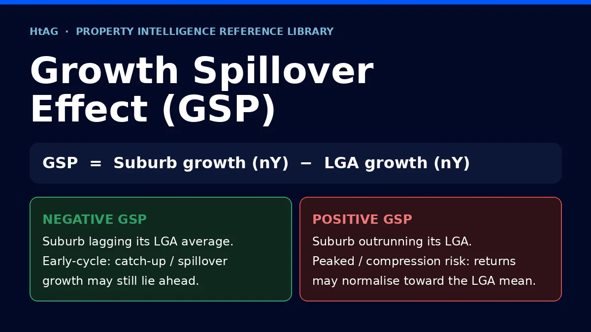
Growth Spillover Effect (GSP) is a property metric that measures the gap between a suburb’s capital growth and the average growth of its surrounding Local Government Area (LGA), across multiple timeframes. According to HtAG Analytics, GSP is calculated as the suburb’s growth minus its LGA’s growth over the same 3, 5 and 10-year windows — turning “this suburb grew 8%” into the far more decision-useful “this suburb grew 4 percentage points faster than everything around it.”
The sign is what matters. A negative GSP means a suburb has lagged its council — an early-cycle signal that catch-up, or “spillover”, growth may still lie ahead. A positive GSP means a suburb has outrun its neighbours — a sign growth has concentrated there and returns may normalise back toward the local mean.
GSP detects compression — the moment growth stops spreading across a council and starts concentrating in a single suburb. Negative GSP suburbs are the ones the spillover has not yet reached.
HtAG Analytics, Property Intelligence Reference Library
If You Remember One Thing
If You Remember One Thing
Growth that has spread to every suburb in a council has usually already happened. GSP helps you find the suburbs the wave has not reached yet — the negative-GSP laggards sitting next to streets that have already run.
How GSP Works: Suburb Growth Minus LGA Growth
GSP works by re-basing a suburb’s performance against its own backyard. Instead of comparing a suburb to the whole state or nation, it compares it to the council it belongs to — the set of suburbs that share the same employment catchment, infrastructure pipeline and broad price band.
The logic is straightforward: capital growth tends to ripple outward from the strongest pockets of a council to the cheaper or overlooked ones. When one suburb races ahead of its LGA, the price gap to neighbouring suburbs widens — and buyers priced out of the leader start looking next door. That is the spillover GSP is named for.
What This Means in Plain English
Think of a council area as a street of houses being repainted one by one. If only the corner house is freshly painted, the others still have room to catch up. If every house on the street is already done, the easy gains are behind you. GSP measures how much “repainting” is left.
Reading the sign and the timeframe
GSP is reported across 3, 5 and 10-year horizons because the story can differ by timeframe. A suburb can be negative on a 3-year view (recently lagging) but positive on 10 years (a long-run outperformer catching its breath). Reading all three together tells you whether you are looking at a structural laggard, a temporary pause, or a market that has genuinely topped relative to its peers.
In HtAG’s decile rankings the ordering is deliberately reversed: lagging, negative-GSP suburbs score higher, because the metric is built to surface opportunity that headline growth tables hide. This mirrors how the related Growth Pattern Deviation (GPD) metric treats negative readings as favourable.
A Real GSP Worked Example: Three Suburbs, One Council
The clearest way to understand GSP is to watch it separate three suburbs inside a single council. The table below uses current HtAG Analytics house data for Frankston City (VIC) to 31 May 2026 — the LGA and three of its suburbs, on 3-year annualised growth.
| Area (houses) | 3yr growth p.a. | vs LGA (GSP) | Signal |
|---|---|---|---|
| Frankston City (LGA benchmark) | 4.27% | — | Benchmark |
| Frankston South | 3.24% | −1.03 pp | Negative → early-cycle |
| Frankston | 5.61% | +1.34 pp | Mild positive |
| Frankston North | 8.42% | +4.15 pp | Positive → compression |
Source: HtAG Analytics, house market data to 31 May 2026. GSP shown as the suburb’s 3-year annualised growth minus the LGA’s, in percentage points (pp).
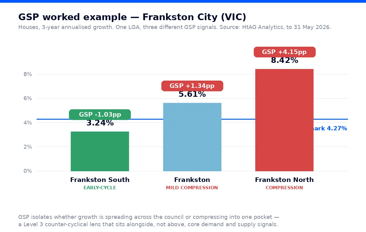
Three suburbs, one council, three different stories. Frankston North has grown 8.42% a year — more than four percentage points above its LGA. That is a strongly positive GSP: the spillover has already arrived, and on a relative basis the easy gains may be behind it. Its 18.6% one-year surge underlines how far it has run.
Frankston South, the premium pocket, tells the opposite story. At 3.24% a year it sits roughly a point below its council — a negative GSP. Read in isolation that looks like weakness; read through the GSP lens it flags a suburb the local growth wave has not yet fully reached. Frankston itself sits in between, mildly ahead of the pack.
What This Means in Plain English
In Frankston City, the cheapest pocket (Frankston North) has already had the big run, while the dearest pocket (Frankston South) has lagged the council. GSP does not tell you to buy or avoid either — it tells you where in the local cycle each one sits, so you can ask better questions before you do.
GPD vs GSP: Two Counter-Cyclical Siblings
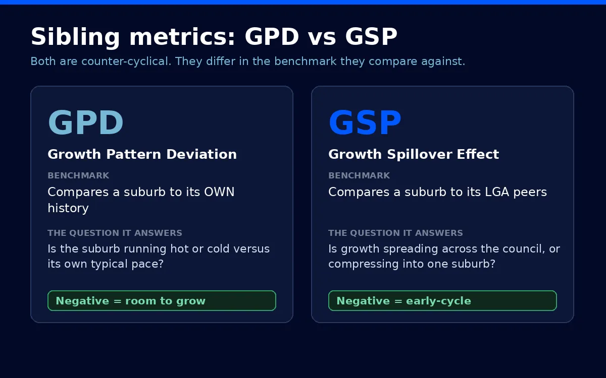
GPD and GSP are siblings — both counter-cyclical, both treating negative readings as favourable — but they answer different questions because they use different benchmarks. Growth Pattern Deviation (GPD) compares a suburb to its own history. GSP compares a suburb to its LGA peers.
| Dimension | GPD — Growth Pattern Deviation | GSP — Growth Spillover Effect |
|---|---|---|
| Compares against | The suburb’s own historical growth | The surrounding LGA’s growth |
| Detects | Whether a suburb is running hot or cold vs its own pace | Whether growth is spreading or compressing geographically |
| Favourable signal | Negative (lagging own history) | Negative (lagging LGA average) |
| Risk when positive | Cycle peak / deceleration risk | Compression / normalisation risk |
Used together they triangulate. A suburb that is negative on both — quiet versus its own history and lagging its council — is a stronger early-cycle candidate than one flashing only a single signal. For more on why council-level averages can mislead on their own, see our breakdown of LGA vs suburb data.
How to Use GSP Without Getting Burned
Use GSP as a context layer, not a buy signal. Here is the disciplined way to apply it:
- Confirm the core signals first. Establish demand, supply and cycle position using primary metrics like the Growth Rate Cycle (GRC). GSP only adds nuance once the fundamentals stack up.
- Read negative GSP as a question, not an answer. A lagging suburb is worth investigating — but a suburb can lag its LGA because it is genuinely weaker (public housing concentration, flood overlay, poor access), not just early. Check why.
- Cross-check all three timeframes. A negative 3-year GSP on a suburb that is positive over 10 years is a pause; negative across all three may be structural.
- Pair it with GPD. Two counter-cyclical signals pointing the same way is far stronger than one.
- Mind the price gap. Spillover works when a leader has pulled meaningfully ahead. If the laggard is cheaper for a permanent reason, the gap may never close.
Common Mistakes When Reading GSP
- Treating negative GSP as an automatic buy. It is a flag to investigate, not a recommendation. Weak suburbs lag for real reasons.
- Using GSP as a headline ranking. It is a Level 3 contextual indicator — it should never outrank demand, supply or affordability evidence.
- Ignoring the LGA boundary. Some councils are huge and economically mixed; the “average” can blur very different sub-markets. Always sanity-check the council’s internal spread.
- Reading one timeframe in isolation. The 3, 5 and 10-year views exist to be read together.
Research Note
In HtAG’s testing, GSP earns its keep as a tie-breaker and context layer rather than a standalone predictor — most powerful when a negative reading coincides with independent demand and supply strength. We publish what the signal means, not the calibration behind it.
Where GSP Sits in the HtAG Decision Stack
GSP is a Level 3 — contextual and supplementary — counter-cyclical indicator. Level 1 and Level 2 metrics (demand depth, supply tightness, cycle position, affordability) carry the weight of a decision. GSP, like GPD, adds geographic nuance on top: it tells you where a suburb sits relative to its neighbours, which can sharpen timing and conviction once the fundamentals are confirmed.
This layered approach is the backbone of property intelligence — turning raw growth numbers into scored, ranked, decision-grade signals. You can see GSP and its siblings mapped across the country on the GeoDex suburb heatmap, and validated against outcomes in the Evidence Portal.
The conceptual framework behind this metric is published openly for transparency and education. Its proprietary implementation — calibration, weighting, validation and the underlying data — remains the confidential intellectual property of HtAG Analytics.
Surface This Data Inside Your AI Agent
The HtAG Developer Portal now exposes the data described in this article — and every other HtAG dataset — through MCP (Model Context Protocol) connectors. Investors and buyers’ agents using Claude, Perplexity, Manus AI, ChatGPT (via custom connectors) or any other MCP-compatible AI agent can query HtAG growth and spillover data directly inside the AI tool they already use.
HtAG’s MCP-enabled Developer Portal puts every metric in this article inside your AI agent. Apply for access and run the full GSP analysis on any Australian council without leaving Claude or Perplexity.
HtAG Analytics Developer Portal (2026)
Browse the endpoint catalogue at developer.htagai.com and submit the HtAG Developer Portal application — approved members receive an API key and an MCP setup guide for their preferred AI tool.
From Data Signal to Portfolio Decision
The GSP, GPD and GRC metrics described in this article are live inside the HtAG Analytics platform — updated each quarter as new valuation data flows in. Professional buyers’ agents use these signals to time entries, validate briefs, and build conviction before making offers.
If you’re building a portfolio and want to see the exact data powering articles like this one — including current GSP readings for every Australian council — the HtAG Starter Plan gives you suburb-level analytics across every market, with no lock-in.
Start your HtAG Analytics membership → · Apply for Developer Portal access →
Key Takeaways
- GSP = suburb growth minus LGA growth, across 3, 5 and 10-year windows. It re-bases a suburb against its own council.
- Negative GSP = early-cycle. The suburb lags its council — spillover growth may still lie ahead.
- Positive GSP = compression risk. The suburb has outrun its peers; returns may normalise toward the LGA mean.
- In Frankston City, Frankston North ran +4.15pp ahead of its LGA while Frankston South sat −1.03pp behind — three GSP stories in one council.
- GSP is a Level 3 context layer, strongest paired with GPD and confirmed by core demand and supply signals — never used alone.
Frequently Asked Questions
What is Growth Spillover Effect (GSP) in property?
Growth Spillover Effect (GSP) is a metric that compares a suburb’s capital growth to the average growth of its surrounding Local Government Area over 3, 5 and 10 years. A negative GSP means the suburb has lagged its council (an early-cycle signal); a positive GSP means it has outrun its peers (a compression-risk signal).
Is a negative GSP good or bad?
In HtAG’s framework a negative GSP is treated as favourable — it flags a suburb that has lagged its council and may still benefit from spillover growth. But it is a question to investigate, not an automatic buy: some suburbs lag for structural reasons. GSP is a Level 3 contextual indicator, used alongside core demand and supply metrics.
What is the difference between GSP and GPD?
GPD (Growth Pattern Deviation) compares a suburb to its own historical growth; GSP (Growth Spillover Effect) compares a suburb to its LGA peers. GPD detects whether a suburb is running hot or cold versus its own pace; GSP detects whether growth is spreading across a council or compressing into one suburb. Both treat negative readings as favourable.
How do I access HtAG GSP data inside Claude or Perplexity?
HtAG exposes its growth and spillover data through the Developer Portal’s MCP (Model Context Protocol) connectors. Browse the endpoint catalogue at https://developer.htagai.com/ and apply for access at https://links.htag.com.au/widget/form/GFVegAaXzeTUH7QzRl1T. Approved members receive an API key and an MCP setup guide so they can query HtAG data directly inside Claude, Perplexity, Manus AI or any MCP-compatible agent.
Disclaimer: This article is general information only and does not constitute financial, investment or property advice. Property data referenced reflects HtAG Analytics figures to 31 May 2026 and is subject to revision. Past performance is not a reliable indicator of future results. Always conduct your own due diligence and seek licensed professional advice before making an investment decision.
This article forms part of the HtAG Property Intelligence Reference Library — a structured knowledge base documenting the concepts, metrics and methodologies used to analyse Australian residential property markets.
Reference Standard PI-GSP · Version 1.0


